Sample Workflow

This section provides a step-by-step guide on how to run a shoreline change analysis using QSCAT with sample data from Agoo, La Union shorelines. The sample data includes shoreline vectors from 1977, 1988, 2010, and 2022. The process includes generating the baseline vectors, merging the shoreline vectors, and running the shoreline change analysis.

According to the Required Inputs section, the QSCAT requires the two following layers:

1. Shoreline layer

2. Baseline layer

Preparing the shoreline vectors

The tracing of shoreline vectors are out of scope in this guide. However, the shoreline vectors are already provided in the sample data. The shoreline vectors are saved as separate shapefile layers for each year. The shoreline vectors are saved as follows:

1. Agoo 1977 - shoreline vectors from 1977

2. Agoo 1988 - shoreline vectors from 1988

3. Agoo 2010 - shoreline vectors from 2010

4. Agoo 2022 - shoreline vectors from 2022

You can download the sample data from the following link: <insert link>

Generating the baseline vectors

One of the required inputs for the QSCAT is the baseline vectors. Baseline vectors can be created using the following different strategies:

1. Creating a buffer of merged shorelines layer.

2. Creating a buffer of a single shoreline layer.

3. Manually drawing lines using Add Line Feature.

In this guide, we will choose the first strategy, which is creating a buffer of the merged shorelines layer. Then, we will choose the part of the buffer that best represents the baseline.

Merging the shoreline vectors

Merging the shoreline step is optional. We only apply this if our digitized shorelines are saved as separate shapefile layers. However, in this guide, the Agoo, La Union shorelines are shared as separate shapefile layers. Thus, we will demonstrate here on how to merge these layers.

However, regardless on what strategy you choose for generating the baseline vectors, the QSCAT requires the shoreline layers to be merged into a single layer. Also, if you choose the first strategy, you should first merge the shoreline layers so that we can create a buffer of all shorelines.

1. Open Processing Toolbox via Processing ‣ Toolbox.

   

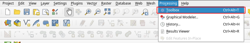
   Fig. 44 Opening Processing Toolbox in QGIS

   
   

2. Search Merge vector layers in the search bar. Then double left-click on Merge vector layers to open the tool.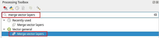

   

   Fig. 45 Searching merge vector layers in Processing Toolbox

   
   

3. In Input layers, click … then select the all shoreline layers to be merged. In this example, select Agoo 1977, Agoo 1988, Agoo 2010, and Agoo 2022. After you are done selecting, click OK.

   

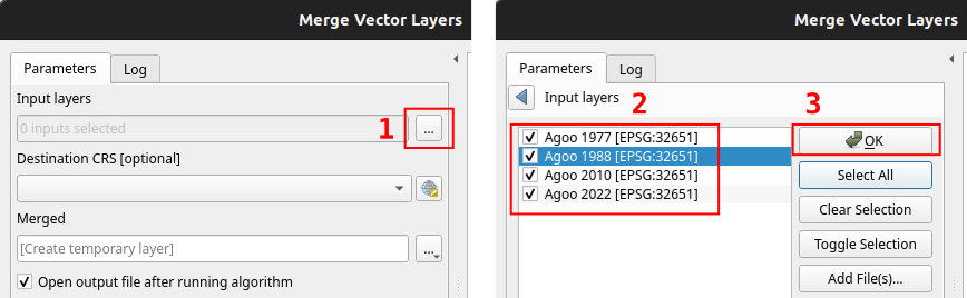
   Fig. 46 Selecting input layers to be merged

   
   

4. In Destination CRS, select the appropriate CRS of the shoreline layers for your project. In this example, select EPSG:32651.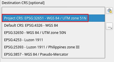

   

   Fig. 47 Choosing destination CRS

   
   

5. In Merged, it is recommended to permanently save the merged layers. Thus, click …, and Save to file. Choose a folder (recommended in the same folder of your QGIS project), pick a file name such as Shorelines Merged and choose SHP files (*.shp) as the file type, and click Save. Click Run to start the merge process, then you can Close.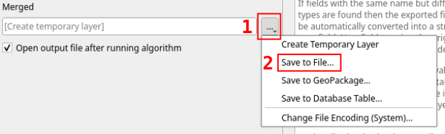

   

   Fig. 48 Opening Save to file dialog

   
   

   

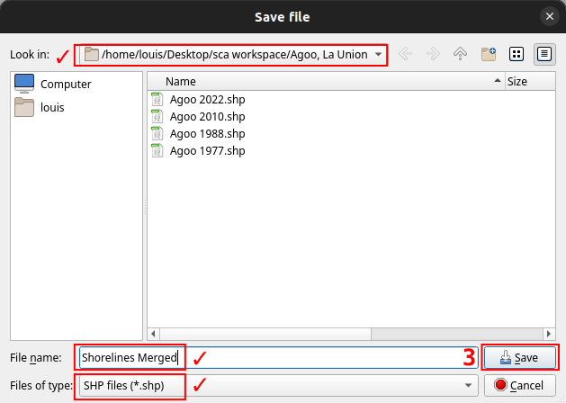
   Fig. 49 Saving merged vector layer

   
   

   

   
   

   

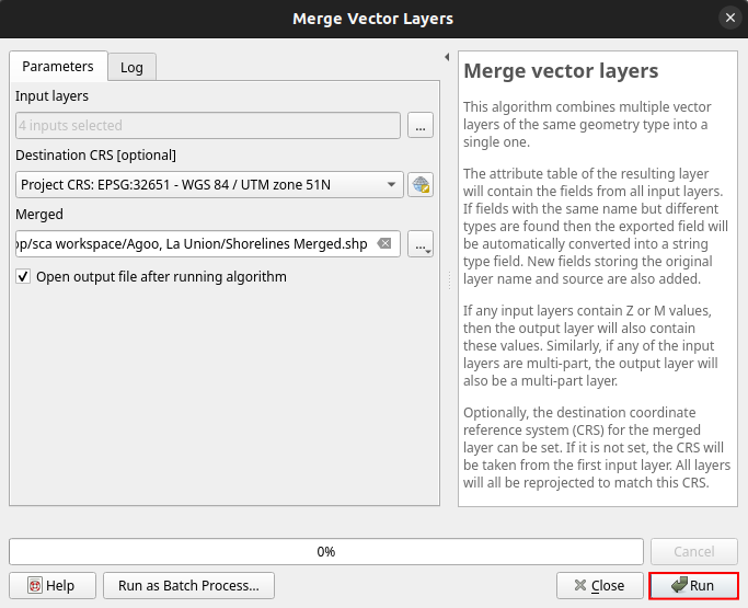
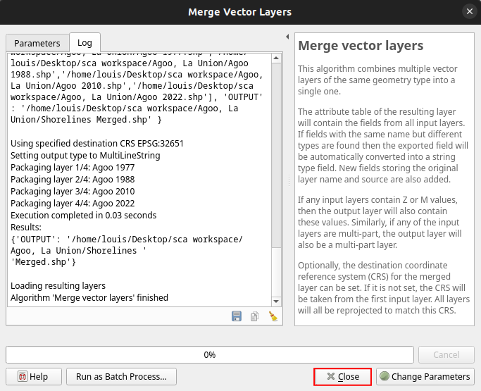
   Fig. 50 Closing merge vector layers

   
   

6. Once finished, the newly merged layer with your chosen file name will appear in the Layers panel.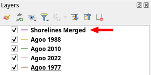

   

   Fig. 51 Showing saved merged vector layer

   
   

Creating a buffer using QSCAT

Here, we can start using the QSCAT plugin. The QSCAT plugin has a feature that automates the creation of the Baseline buffer.

1. Open QSCAT if not yet opened. The QSCAT plugin can be open by clicking the icon at the top toolbar area near the Python Console icon.

2. In the QSCAT interface, navigate to Automator Tab. Then, in the Baseline Buffer section, select the merged shoreline layer from Input shorelines layer. Next, enter 400 in the Distance (m), click Buffer. The buffer will be created and displayed in the map canvas. The buffer will be saved as a temporary layer.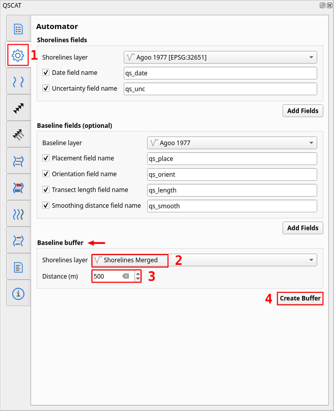

   

   Fig. 52 Creating baseline buffer in Automator Tab

   
   

   

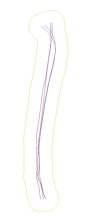
   Fig. 53 Created buffer on merged shoreline with 400 meters distance

   
   

Converting the buffer to baseline vector

1. First, enable the Advanced Digitizing Toolbar (if not yet enabled) by going to View ‣ Toolbars ‣ Advanced Digitizing Toolbar.

   

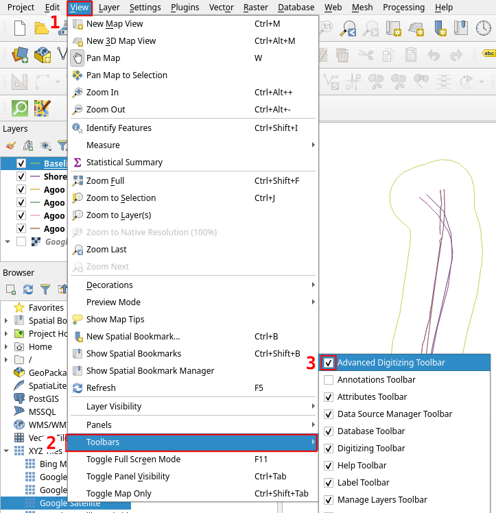
   Fig. 54 Enabling Advanced Digitizing Toolbar

   
   

   

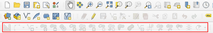
   Fig. 55 Advanced Digitizing Toolbar location

   
   

2. Right click on the baseline buffer layer and select Toggle Editing. The baseline buffer layer will be editable if there is a icon on the layer.

   

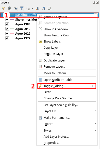
   Fig. 56 Toggling editing of baseline buffer layer

   
   

3. In the Advanced Digitizing Toolbar, click Split Features.

   

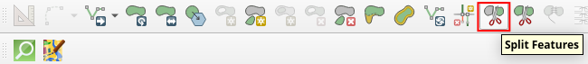
   Fig. 57 Clicking Split Features

   
   

4. Use the Split Features tool to draw two lines that intersects the baseline buffer. First, draw the first line where you want the first split. Then, draw the second line where you want the second split. If drawn properly, the baseline buffer will be split into parts.

   

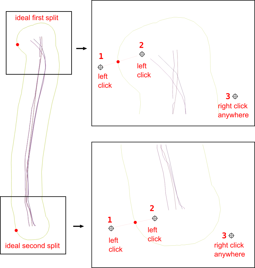
   Fig. 58 Splitting features using Split Features

   
   

5. Next, select Select Features tool and select the baseline buffer segments that you want to remove. Selected segment will be highlighted in yellow line and red points (X). Hit Delete on your keyboard to remove the selected segment. Remove all segments that you do not want until only the baseline segment you want remains.

   

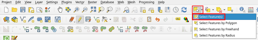
   Fig. 59 Clicking Select Features

   
   

   

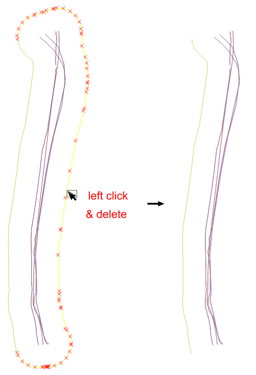
   Fig. 60 Selecting and deleting a feature

   
   

6. Finally, right click on the baseline buffer layer and select Toggle Editing and it will prompt to save the changes.

   Warning

   There will be a case when the baseline buffer are split unexpectedly. As you can see in Fig. 61, you can verify that there are two resulting segments even though we did not draw a line there.

   

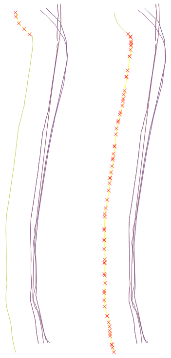
   Fig. 61 Unexpected split of baseline buffer

   
   

   To fix this, go back to the editing mode ( Toggle Editing). Select the two segments by clicking left click on each segment while holding Shift key. Then, in Advanced Digitizing Toolbar, click Merge Selected Features, and click OK. The two segments will be merged into one, you can verify by selecting the features. You can Toggle Editing again to save.

   

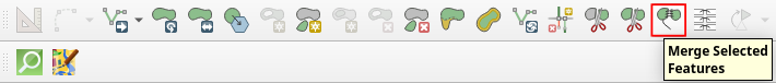
   Fig. 62 Clicking Merge Selected Features

   
   

   

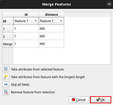
   Fig. 63 Merging Selected Features

   
   

7. If you are okay with the final baseline, you can now permanently save it as a file, right click on the layer and select Export –> Save Features As…. Choose a folder (recommended in the same folder of your QGIS project), pick a file name such as Baseline, and choose ESRI Shapefile (*.shp *.SHP) as the file type, and click Save. Choose appropriate CRS for your project and click OK.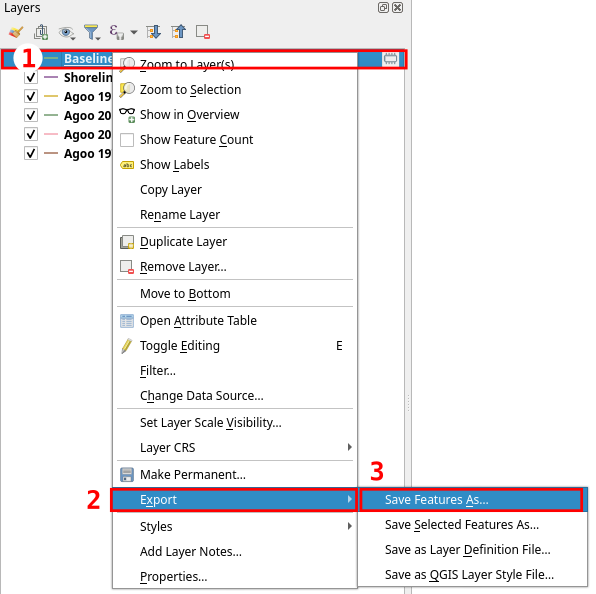

   

   Fig. 64 Accessing Save Feature As…

   
   

   

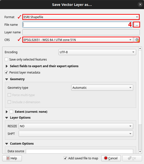
   Fig. 65 Saving Vector Layer As…

   
   

   

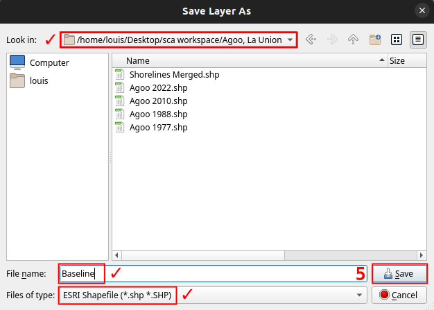
   Fig. 66 Saving Layer As…

   
   

   

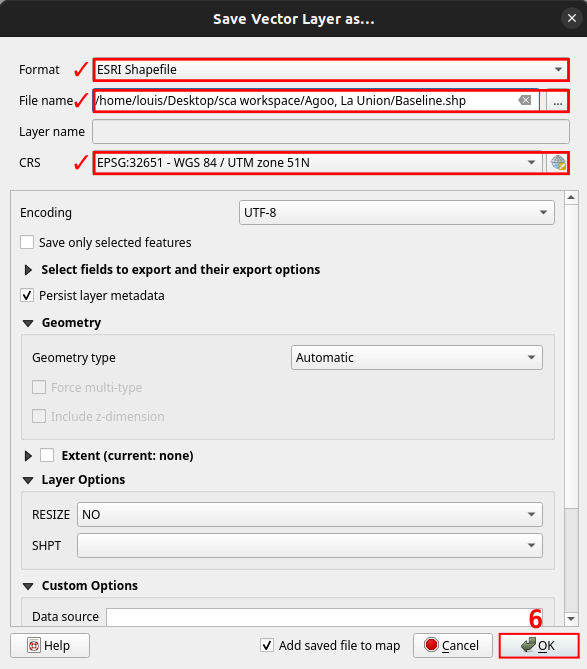
   Fig. 67 Finalizing Saving Vector Layer As…

   
   

Configuring the shoreline and baseline layer attributes

Shorelines

Next, we need to add details of each shoreline such as its date and its uncertainty value of the images. We can use Shoreline fields automator to add the required fields for these.

1. Navigate to Automator Tab. Then, in the Shorelines fields, select the merged shoreline layer from Shorelines layer. Make sure Date field name and Uncertainty field name is both checked. Type the appropriate date field name and uncertainty field name or leave as is. In this example, we choose qs_date and qs_unc as the field names. Click Add Fields.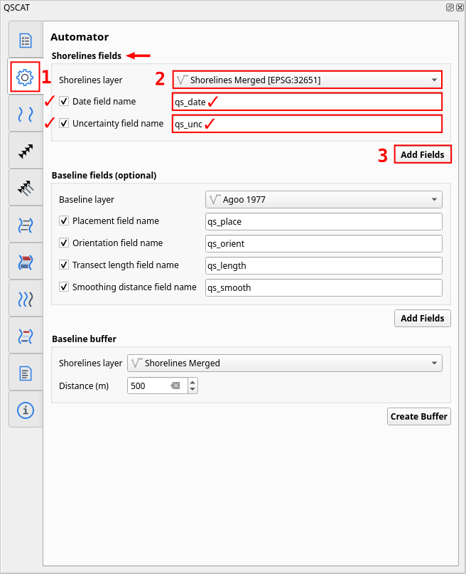

   

   Fig. 68 Automating adding of shoreline fields using Shoreline Fields Automator

   
   

2. Then, we need to fill in the details of each shoreline. Right click on the merged shoreline layer and select Open Attribute Table. But first, enable the Toggle Editing if not yet enabled. In the attribute table, fill in the details of each shoreline such as its date and its uncertainty value. In our sample data, input the following details:

   Table 7 Shoreline date and uncertainty of Agoo, La Union shorelines

   Shoreline	Date	Uncertainty
   Agoo 1977	01/1977	25
   Agoo 1988	03/1988	15
   Agoo 2010	05/2010	15
   Agoo 2022	04/2022	15

   According to Shorelines fields, date is in the format of MM/YYYY and uncertainty is in meters. Also, make sure that details aligns based on the shoreline layer.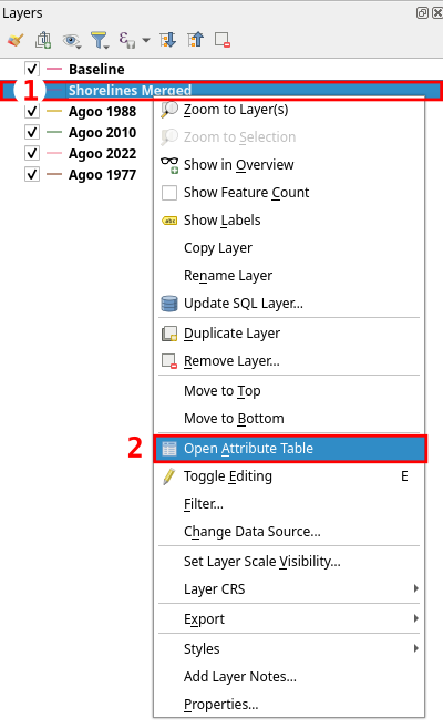

   

   Fig. 69 Opening attribute table of shoreline layer

   
   

   

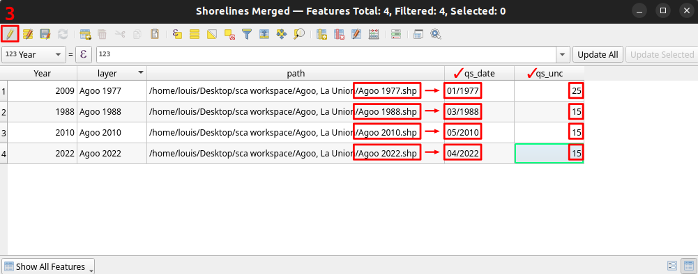
   Fig. 70 Editing attribute table of shoreline layer

   
   

   

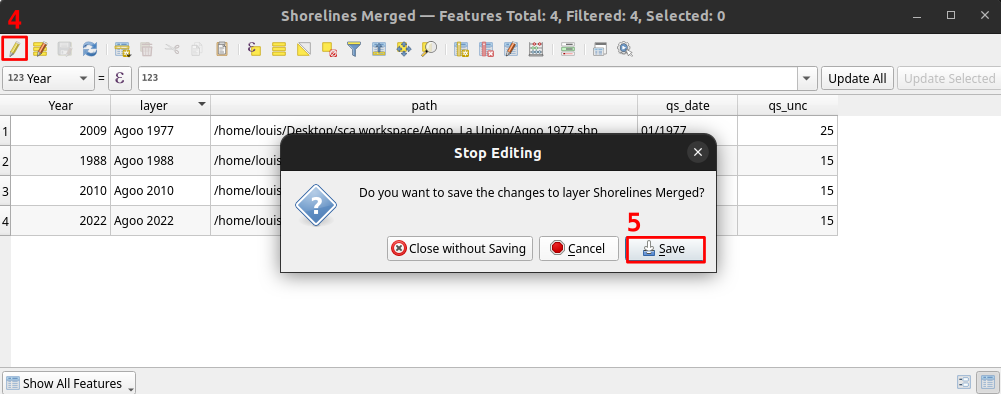
   Fig. 71 Saving attribute table of shoreline layer

   
   

Baseline

Baseline also optionally includes fields such as placement, transect length, and orientation. However for this sample data, we will not add any fields because it is only applicable for multi baseline. For more information, refer to Baseline fields.

Configuring the selections of layer and fields

1. For shorelines, go to Shorelines Tab.

   In Layer section, select the merged shoreline layer as the Input layer. Leave Default data uncertainty as is; this value is used when no uncertainty value is provided in a shoreline uncertainty field (Layer).

   In Fields section, select the added date (Year) and uncertainty (Uncertainty) field names, and click Save.

   

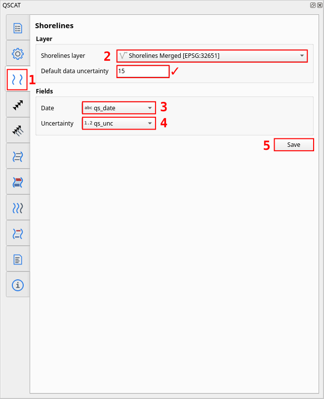
   Fig. 72 Configuring shorelines in Shorelines Tab

   
   

2. For baseline, go to Baseline Tab.

   In Layer section, select the baseline layer as the Input layer.

   In Placement section, select Sea or offshore (see Placement).

   In Orientation section, select Land is to the RIGHT (R) (see Orientation), and click Save.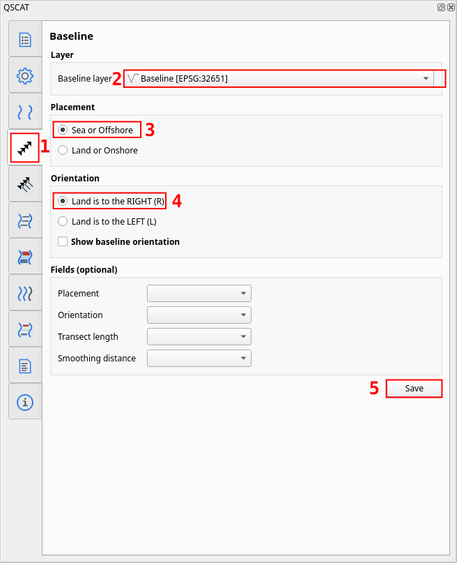

   

   Fig. 73 Configuring baseline in Baseline Tab

   
   

Casting of transects

We can now start the process of running shoreline change analysis. The first step is to cast transects. The transects are lines that are perpendicular to the baseline. The transects are used to measure the shoreline change statistics.

1. Go to Transects Tab.

   In Layer section, select a name for the transect layer in Layer name. In this example, we leave transects as is (see Vector layer output how is the output name used).

   In Count section, select how would you want the number of transects to be determined. In this example, we choose By transect spacing and leave 50 meters as is` (see Count).

   In Parameters section, leave Transect length and Smoothing distance as is (see Parameters).

   Click Cast Transect to start the process of casting transects. The transects will be created and displayed in the map canvas. The transects will be saved as a temporary layer. You can optionally Save the selections such that it will be retain when you close QSCAT or QGIS.

   

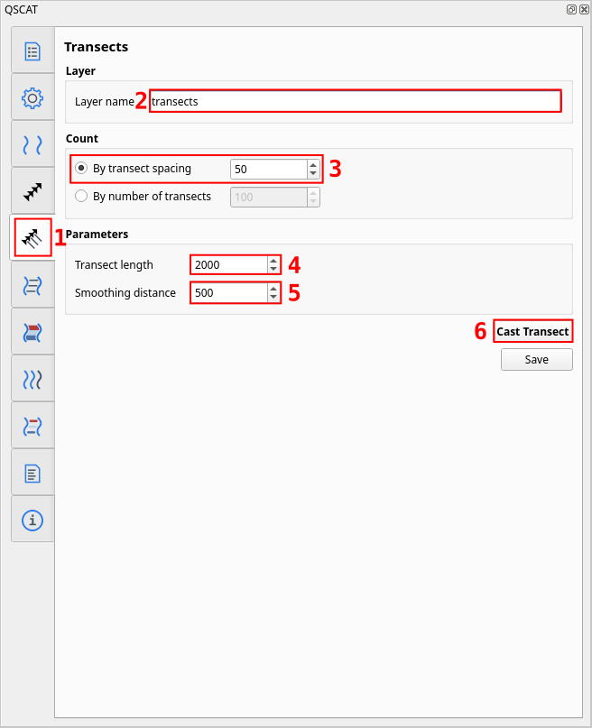
   Fig. 74 Casting transects using Transect Tab

   
   

   

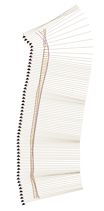
   Fig. 75 Transects with 2000 meters length, and 500 meters smoothing distance together with baseline (baseline orientation shown) and shorelines

   
   

   

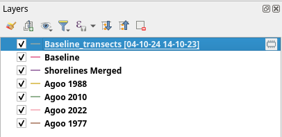
   Fig. 76 Current layers with transects

   
   

Computing the shoreline change

1. Go to Shoreline Change Tab.

   In General section, select the created transect layer (note that after every cast the transects layer will be automatically selected here). You can optionally Clip transects if you want, this is only for visualization purposes and does not affect statistics. For summary reports location (see Tab: Summary Reports).

   In Transect-shoreline intersections, leave Distance and Farthest as is (see Transect-shoreline intersections).

   In Shoreline change statistics, select statistics you want to calculate, select all via Select / Deselect All (see Shoreline change statistics).

   In NSM and EPR dates, make sure to select 04/2022 in Newest date and 01/1977 in Oldest date (see Pairwise comparison of shorelines).

   In Additional parameters, leave Confidence interval (%) as is (see Additional parameters).

   Click Compute Shoreline Change to start the process of computing shoreline change. The shoreline change statistics will be calculated and the transects will be displayed in the map canvas. The statistics will be saved as a temporary layer. You can optionally Save the selections such that it will be retain when you close QSCAT or QGIS (see Vector layer output) for layer outputs.

   

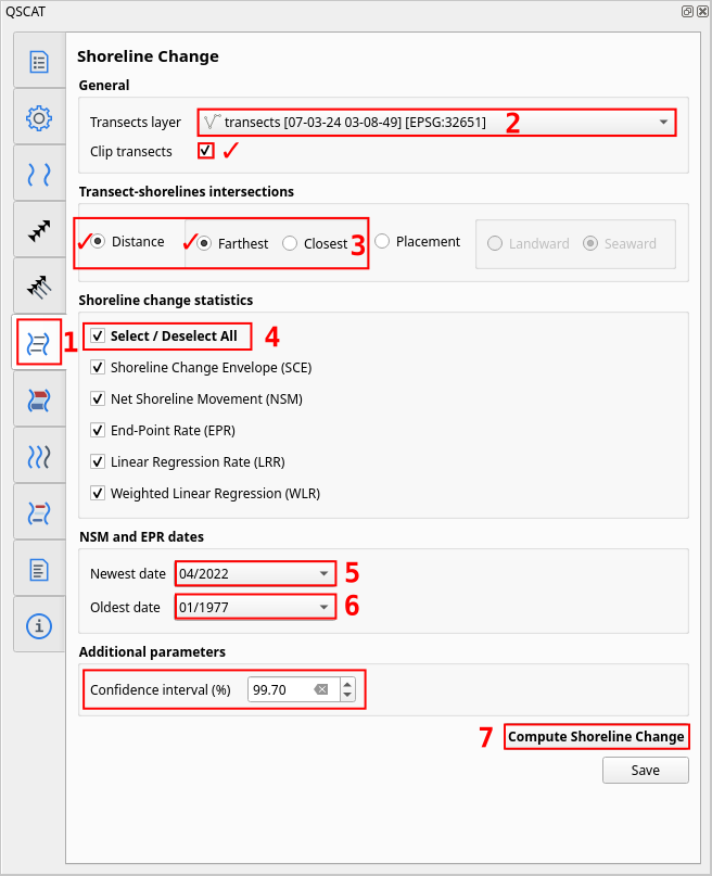
   Fig. 77 Computing shoreline change using Shoreline Change Tab

   
   

   

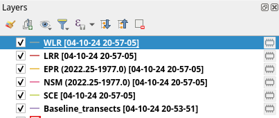
   Fig. 78 Current layers with shoreline change statistics

   
   

   

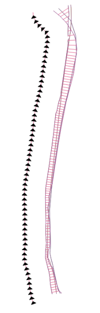
   Fig. 79 Example NSM statistic transect layer when clip transect intersections applied

   
   

   

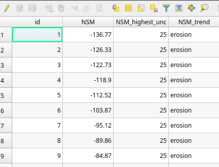
   Fig. 80 Example NSM statistic table field and values

   
   

Running optional features

Computing the area change

This feature requires a polygon area to encompass which would you like to get the area change. Usually, we designed this for a specific area of interest like municipality or barangay boundaries. If you want to get the area change on whole area at once then you can draw a polygon that encompasses the whole area. For this sample data, we will get the area change on the whole area.

Creating the polygon using QGIS

1. In the top part of QGIS, click New Shapefile Layer.

   

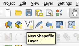
   Fig. 81 Opening New Shapefile Layer

   
   

2. In the File name click …, select a folder location, type a file name such as whole area.shp and Save.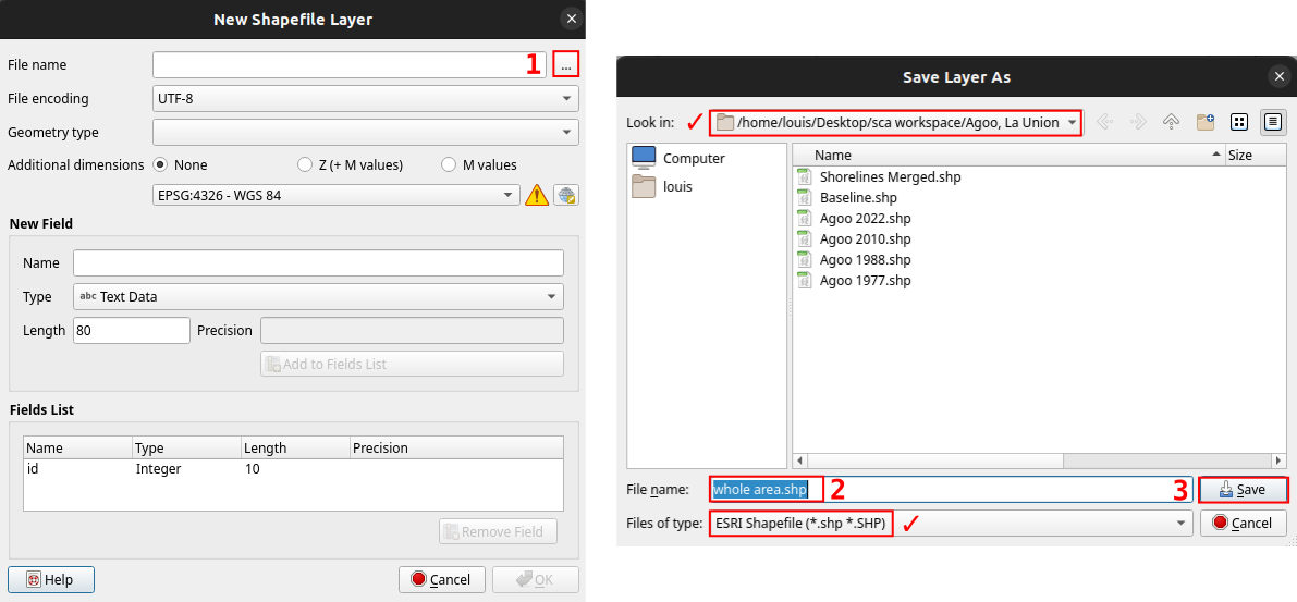

   

   Fig. 82 Saving New Shapefile Layer

   
   

3. Select Polygon as the Geometry type. Select ESPG:32651 and click OK.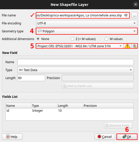

   

   Fig. 83 Final Saving New Shapefile Layer

   
   

4. Change the symbology for better visualization. Double left click the square from left of the layer name. Then, select outline red click Apply and OK.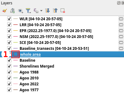

   

   Fig. 84 Opening symbology in layer properties

   
   

   

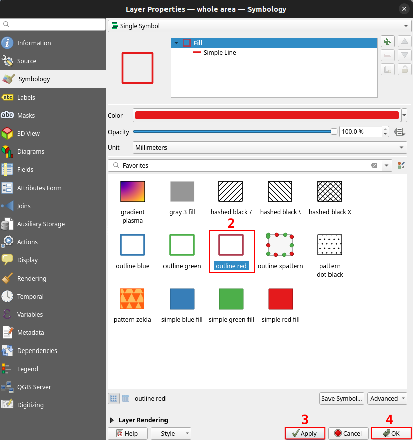
   Fig. 85 Changing symbology in layer properties

   
   

5. Draw the polygon. Toggle the layer to be editable by Toggle Editing. Then, click Add Polygon Feature and draw the polygon that encompasses the whole area. You can draw the polygon with just 4 points enough to cover the whole area. draw 4 points, then right click anywhere to end drawing, and click OK. Of course, you do not need to follow the points on the figure just make sure the polygon will encompass the area of interest. Select Toggle Editing to save the changes.

   

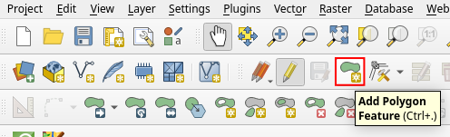
   Fig. 86 Opening Add Polygon Feature

   
   

   

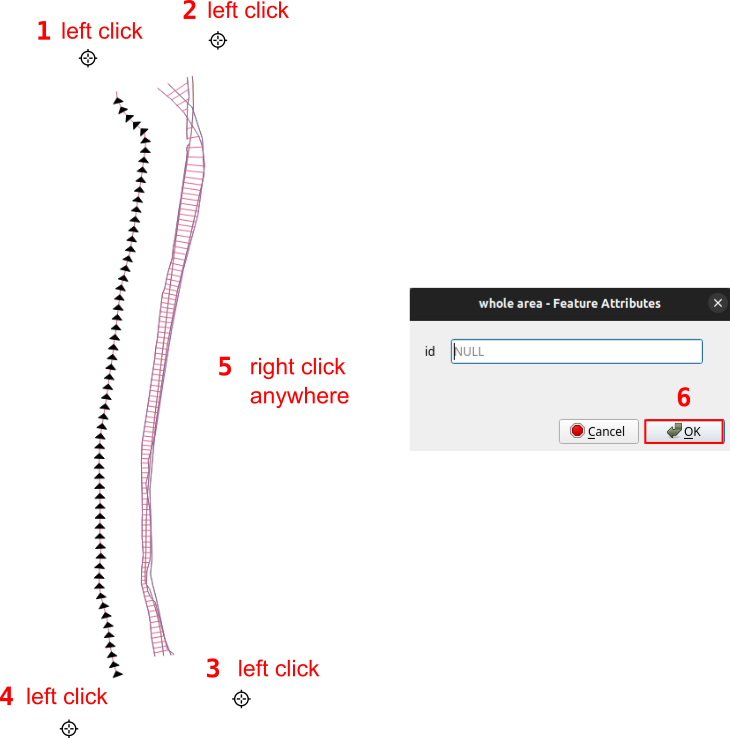
   Fig. 87 Drawing Polygon using Add Polygon Feature

   
   

   

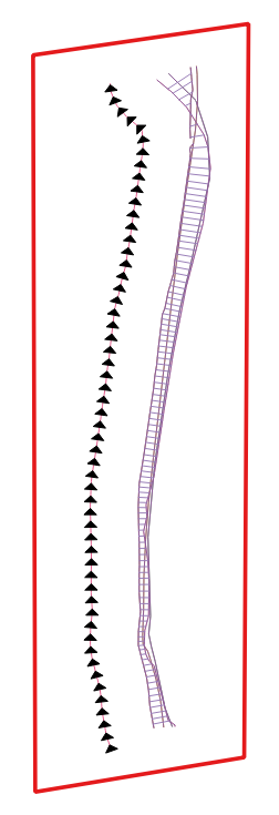
   Fig. 88 Example drawn polygon feature

   
   

6. Go to Area Change Tab.

   In General section, select the created polygon layer as the Polygon layer, and in Shoreline change statistic layer, select the NSM layer. Only NSM and EPR statistics are available for area change for now (see Tab: Area Change).

   

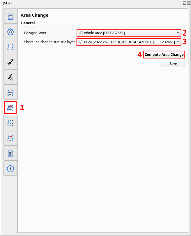
   Fig. 89 Computing area change in Area Change Tab

   
   

   

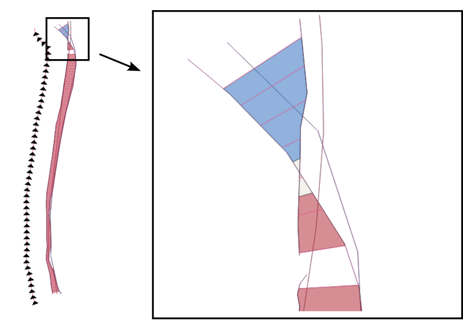
   Fig. 90 Example area change in the top part

   
   

Running the forecasting

1. Go to Forecasting Tab

   In Layer, select the transects layer as the Transects layer.

   In Algorithm, the current available algorithm is Kalman Filter (see Algorithm).

   In Time Period, select 10 years (see Time period) and click Forecast.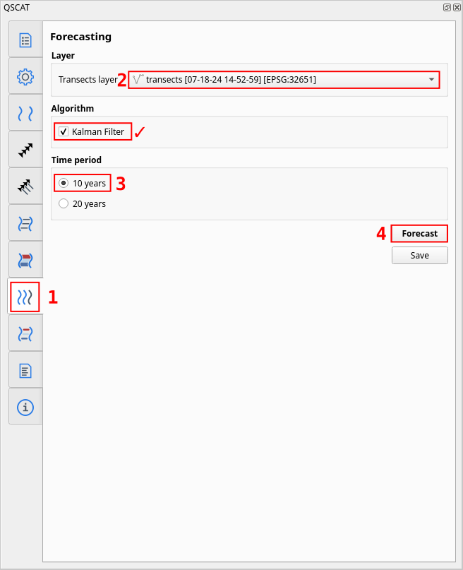

   

   Fig. 91 Forecasting in Forecasting Tab

   
   

   

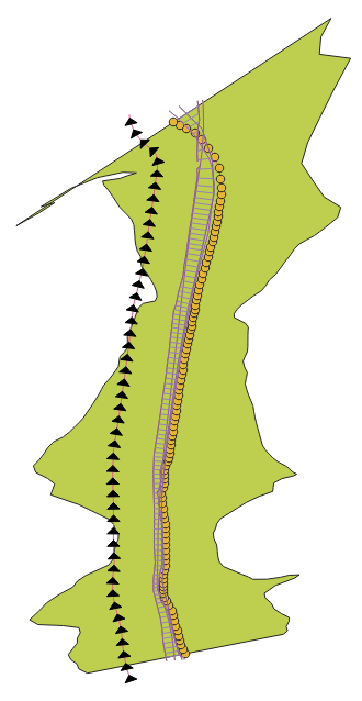
   Fig. 92 Example forecasting in Forecasting Tab

   
   

Visualizing the statistics transects

1. Go to Visualization Tab

   In Layer, select a statistic layer to apply visualization in Shoreline change statistic layer. In this example, we choose the NSM statistic layer. Select the field of NSM layer with the statistic value in Statistic value field, and manually input the value of the uncertainty in Uncertainty value (SCE, NSM, EPR).

   In Color ramp, select Equal Interval as the Mode.Leave the number of Negative classes and Positive classes as is, and click Visualize.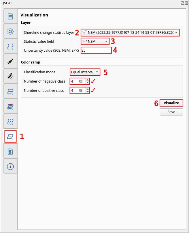

   

   Fig. 93 Visualizing statistics in Visualization Tab

   
   

   

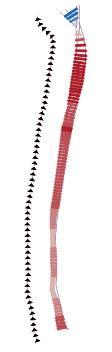
   Fig. 94 Visualized NSM statistic

   
   

   

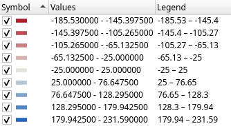
   Fig. 95 Visualized NSM statistic color ramp with equal interval range values